1 Abstract¶

Iterative improvement of LUT through balance forces. Instructions and results.

2 Introduction and Motivation:¶

In this approach we will iteratively improve the LUT. There are two approaches we can follow ‘Applied’ and ‘Balance’ approaches. We will mainly stick with ‘Balance’ but below you see both approaches explanation

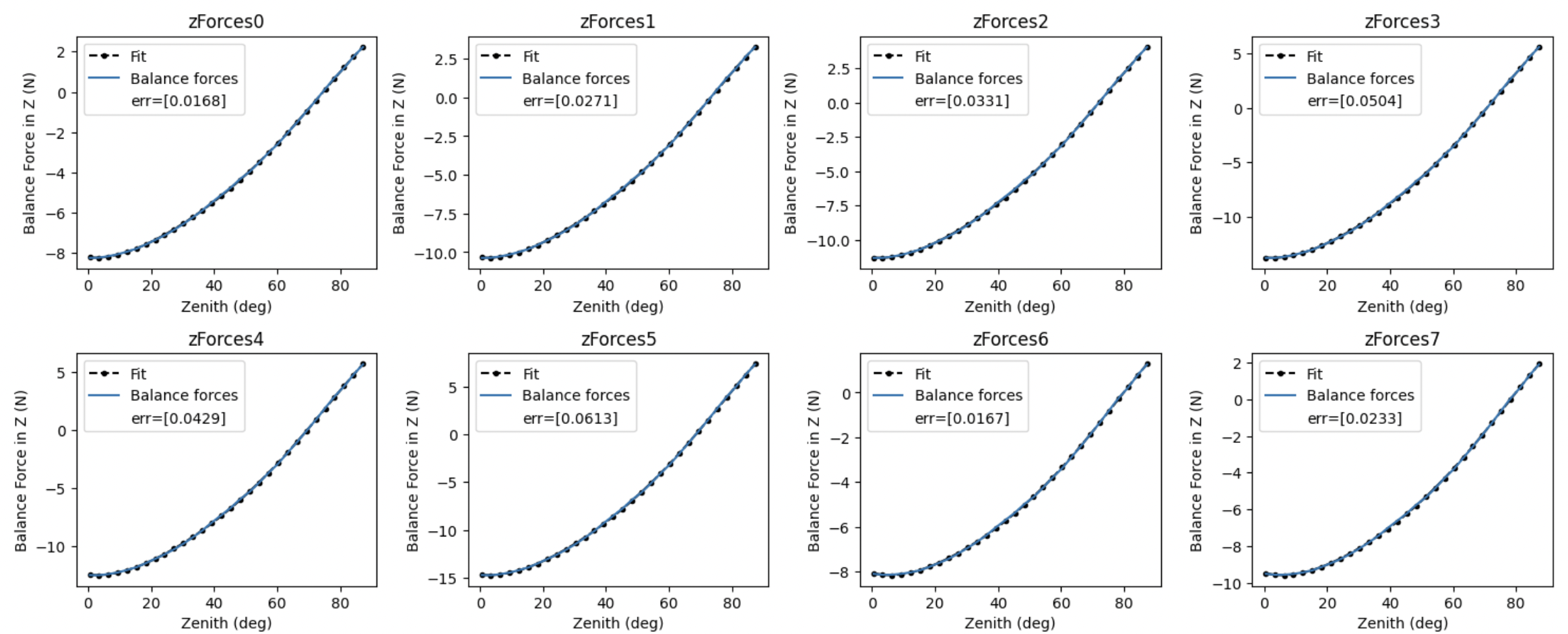
Balance: In this approach we fit the balance forces offsets from the hardpoint correction system with a 5th order polynomial. We add these coefficients to the existing LUT and generate a new csv with the new LUT. The CSV is created at the folder where you have the script.
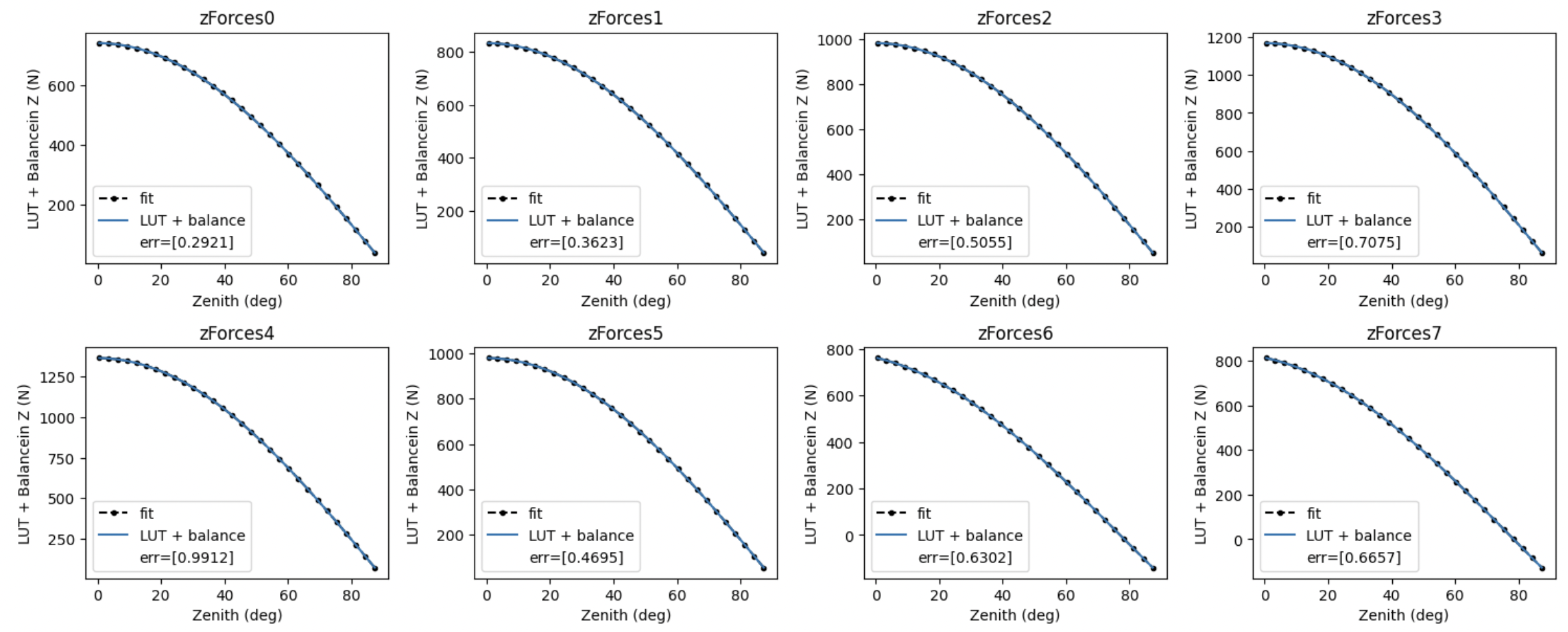
Applied: We look at the Applied forces - Static forces, which is equal to the LUT + Balance forces offsets. We make a fit on these and create a new LUT file, writing from scratch, without relying on the previous LUT.

Note to the reader: when we say 90 - 0 deg we generally refer to 86 deg - 16 deg, the operational range of our telescope.

3 Fitting Balance Forces vs Fitting Applied Forces:¶

We start by showing that we can use either approach to generate the updated LUT. When looking at the data retrieved on 2023-05-31 from 08:35 UTC to 09:05 UTC, with hardpoint corrections enabled (that is, the balance force system). Below is a plot of the two fits that are done to generate the updated LUT:

Balance forces

Applied Forces

The final LUT for the balance force approach is,

Which is approximately the same as the one obtained when using the applied forces approach (See below)

Now that we have shown that both approaches work, we will choose the “Balance force approach” as our baseline and will study the balance forces evolution ss we iteratively update the LUT.

4 LUT Iterative Improvement Results:¶

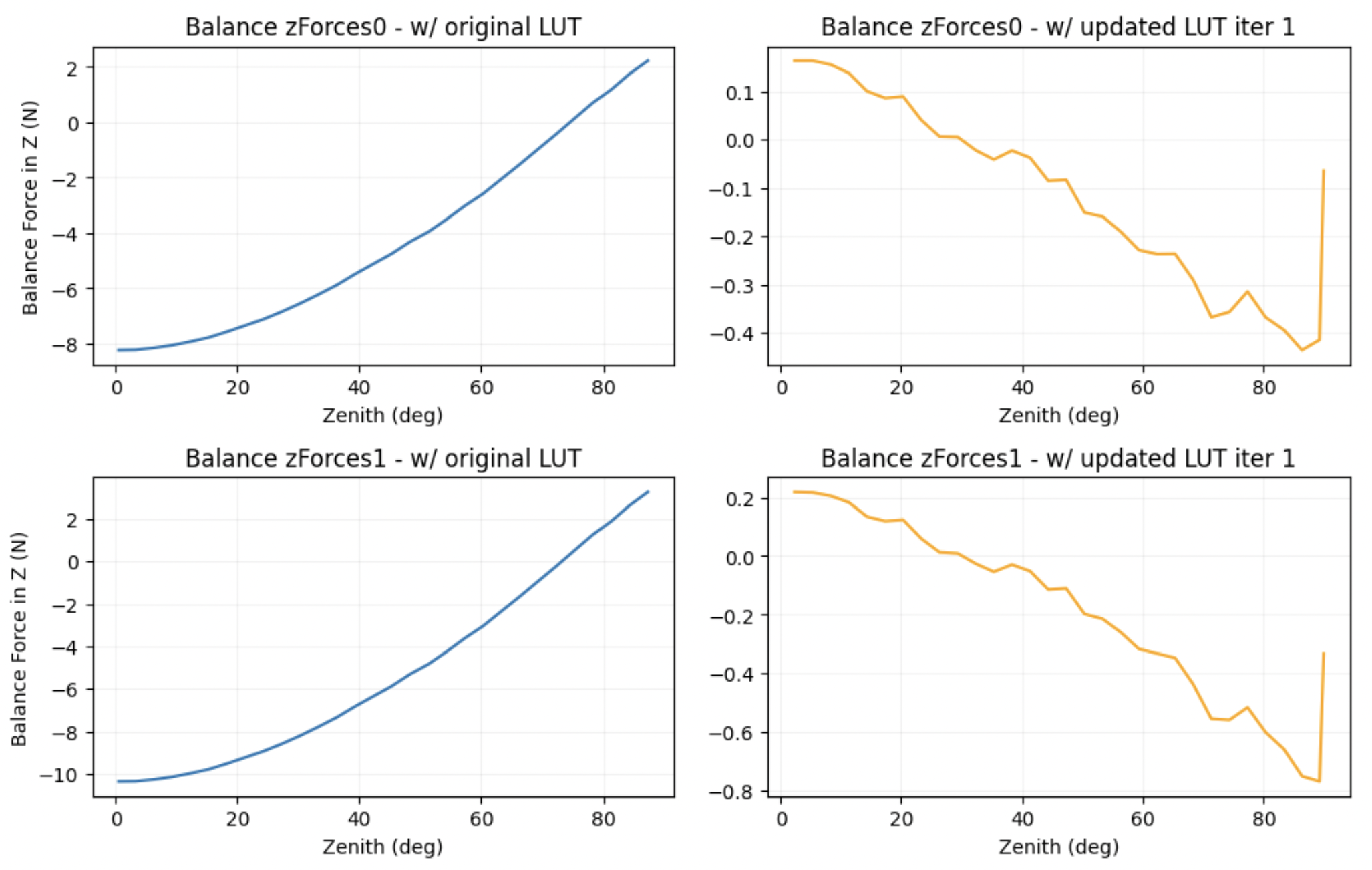
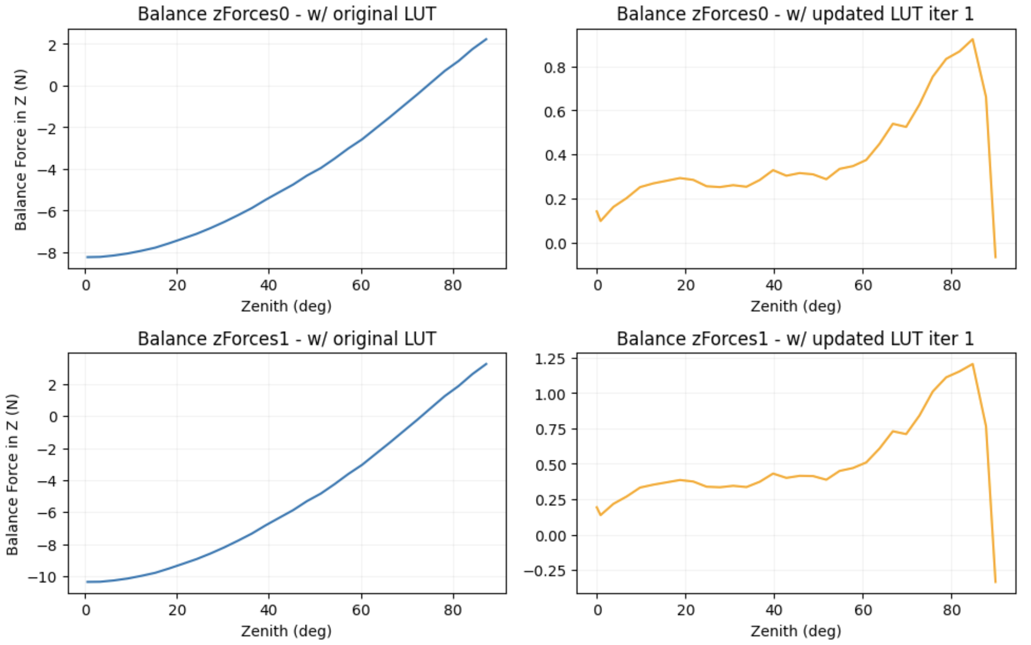
Now we want to look at the evolution of the Balance forces offsets after updating the LUT using the fits discussed in the previous section. We see that the balance forces offsets are reduced by an order of magnitude (to around 0.1 N) after the first LUT improvement iteration.

Z axis balance forces comparison

Y axis balance forces comparison

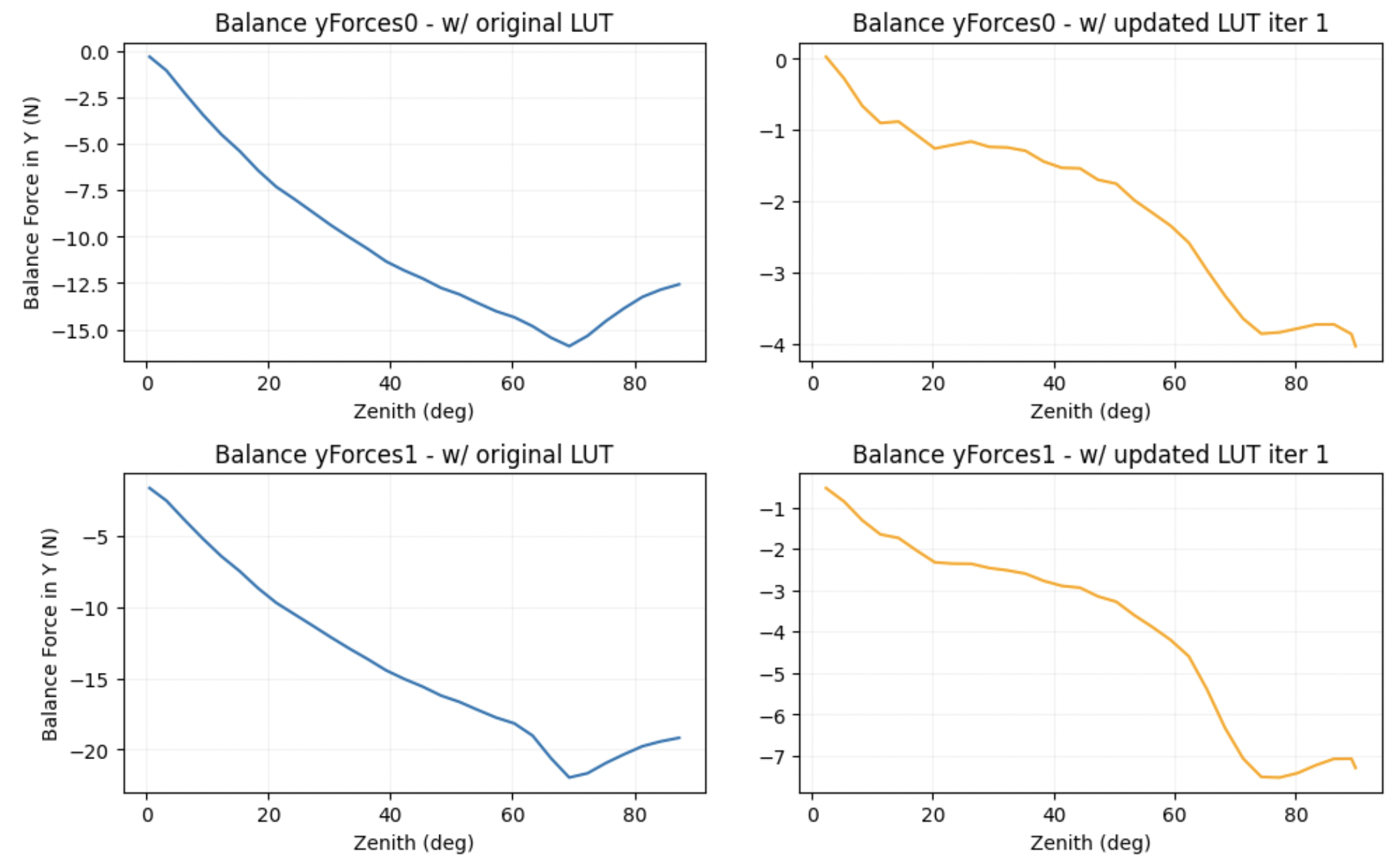
This indicates that our iterative improvement worked in the first iteration. Now we will fit these balance forces again and update the LUT for the second iteration. We are interested in getting to a point in which the balance forces don’t reduce much further. Below are the plots of the fits used for the original balance forces and for the balance forces observed after the first LUT improvement iteration.

Iteration 0 (original) Balance Forces fit

Iteration 1 Balance Forces fit

5 LUT Iterative Improvement - Second LUT iterative update:¶

But, does it make sense to go with the first fit we get from the data? Are the balance forces that we are observing due to a systematic error that we can bring into the LUT or are they at this point just the corrections that the LUT cannot pick up and needs to fall back onto the force balance corrections?

A simple check is to see what are the force balance corrections at another slew from 16 to 86 deg or viceversa, and see if the offsets that we observe are consistent. Below we show the results in Z direction for 16 to 86 deg and from 86 to 16 deg.

From 86 deg to 16 deg.

From 16 deg to 86 deg.

_images/balance_z_comparison_reverse.png

We see that the force balance offsets do not agree on both slews, even though we have the same LUT. This may indicate that we have reached the point in which the LUT cannot be improved further. A wise approach to determine whether this is true or not would be to gather data from multiple slews and plot the force balance mean, median and standard deviation as a function of the zenith angle, to see if there is any systematic error that we can further bring in into the LUT.

6 LUT Iterative Improvement - Tracking coefficient change:¶

At this point, we want to make sure that the coefficient changes that we are applying to the different LUT are getting smaller. We expect the percentage changes to the LUT to decrease at each iteration. We can plot now the results of the percentage change from the previous LUT for the first improvement (iteration 1) and for the second improvement (iteration 2). The second improvement refers to the new fit we got from the balance forces after updating the LUT once. Note that this LUT iteration 2 has not been implemented yet in the system.

We will look at the absolute percentage change for each of the coefficients in the Z direction.

[PLOTS NOT SHOWN HERE PENDING DECISION ON SECOND LUT UPDATE]

7 Instructions (outdated):¶

7.1 Find EFD data to use for LUT improvement¶

Query the EFD to find the start and end time of the data you want to use for LUT improvement. Try to find the exact time where the sweep from 0deg to 90deg (or from 90 deg to 0 deg) started. You will have to select the times in utc.

Here is an example of how you can query and plot the data to find the elevations

start = Time('2023-05-31 08:35:0Z', scale='utc')
end = Time('2023-05-31 09:05:0Z', scale='utc')

# Retrieve elevations
elevations = await client.select_time_series(
   'lsst.sal.MTMount.elevation',
   ['actualPosition', 'timestamp'],
   start,
   end,
)
elevations = elevations['actualPosition'].resample('1T').mean()
elevations.plot()
plt.xlabel('Time (utc)')
plt.ylabel('elevation (deg)')

Once you have chosen the times you want to look at, write them down. You will need them for the next step.

7.2 LUT Improvement Script¶

Clone the ts_aos_utils repository that you can find here Do the following

git clone https://github.com/lsst-ts/ts_aos_utils/

Go to the directory where you cloned the repository and run the script, which is located at python/lsst/ts/aos/utils/scripts
Run the script M1M3LUT.py which will generate a LUT file in the same directory. You can run the script as follows

python3 M1M3LUT.py force_type start_time end_time axis --lut_path --polynomial_degree --resample_rate

# axis = ['X', 'Y', 'Z']
# force_type = ['Balance', 'Applied']
# --lut_path = path to the LUT file you want to improve
# --polynomial_degree = degree of the polynomial you want to fit the data to
# --resample_rate = resample rate of the data you want to use for the LUT improvement.

You will not have to change the polynomial degree or the resample rate. The default values are 5 and 1T respectively.
An example below:

python3 M1M3LUT.py 'Balance' '2023-05-31 08:35:0Z' '2023-05-31 09:05:0Z' 'X' --lut_path="path/to/ts_m1m3support/SettingFiles/Tables/"

7.3 Updating the LUT in cRIO¶

You need to copy the new tables to M1M3 cRIO. cRIO address is m1m3-crio-ss.cp.lsst.org, it’s running a modified Linux, so common linux command works.

Login

username: admin

password: stored in LSST maintel vault in 1password

Copy files to m1m3-crio-ss.cp.lsst.org in the directory /var/lib/M1M3support/Tables. Use scp to copy them.
Save them as Elevation{XYZ}Table.csv, where {XYZ} shall be replaced with axis of the table modified. It’s better to scp to tmp directory first, verify that the files arrive properly, and only after that ssh into m1m3-crio-ss and copy the file from /tmp to /var/lib/M1M3support/Tables:

scp Elevation*Table.csv admin@m1m3-crio-ss.cp.lsst.org:/tmp

Then copy the files from ssh:

ssh admin@m1m3-crio-ss.cp.lsst.org

cp /tmp/Elevatoion*Table.csv /var/lib/M1M3support/v1/tables/

Once done, just cycle M1M3 CSC to standby and bring it back to online. The new table is loaded during start step.

8 Test rundown:¶

Hardpoint corrections should be ON
Do a 0 to 90 deg with balance forces turned on.
Find times in EFD data to use for LUT improvement
Run the script to generate a new LUT file for Z, Y and X axis. You will have to run the script three times. You can choose ‘Balance’ type to start with.
Update the cRIO
Cycle M1M3 CSC to standby and bring it back to online. The new table is now loaded during start step.
Do a 0 to 90 deg (or 90deg to 0 deg) sweep again and repeat the previous steps. Remember that when you run the LUT script, you will have to update the lut_path to point at your previous LUT file.
Do this 5 times.

SITCOMTN-079: Iterative improvement of LUT through balance forces