1 Abstract
This technote summarizes the improvement procedure and results used to update the Look-Up Table (LUT) of M1M3 during the first static and semi-dynamic tests. Here, we describe the basis of the iterative improvement, how it was actually implemented, and report the overall results of the improvement procedure. Additionally, we also provide instructions on how to run the iterative improvement scripts.
2 Introduction and Motivation
Let us first recall what the force balance offsets come from. The Force Balance offsets are determined through the forces measured in the load cells in the mirror’s position defining units (hard points). These are the net forces/moment in the six degrees of freedom resulting from the imbalance between the LUT forces and the forces acting on the mirror. These forces are counteracted by distributing forces through the figure control actuators which are applied to the LUT values as FB offsets. Since the new FB offsets are determined in the presence of existing FB offset, the new FB offsets must be combined with the previous FB offsets. Since the system is deterministic, the Force Balance offset will likely be a simple linear addition.
The assumption that let us improve the initial LUT is that a fraction of the balance forces offsets that was being applied to correct for the harpoint actuator measurements was a fixed offset that could be injected into the LUT. Therefore, the iterative improvement of the LUT can be performed through two different approaches, which we will call ‘Applied forces’ and ‘Balance forces’ approaches.
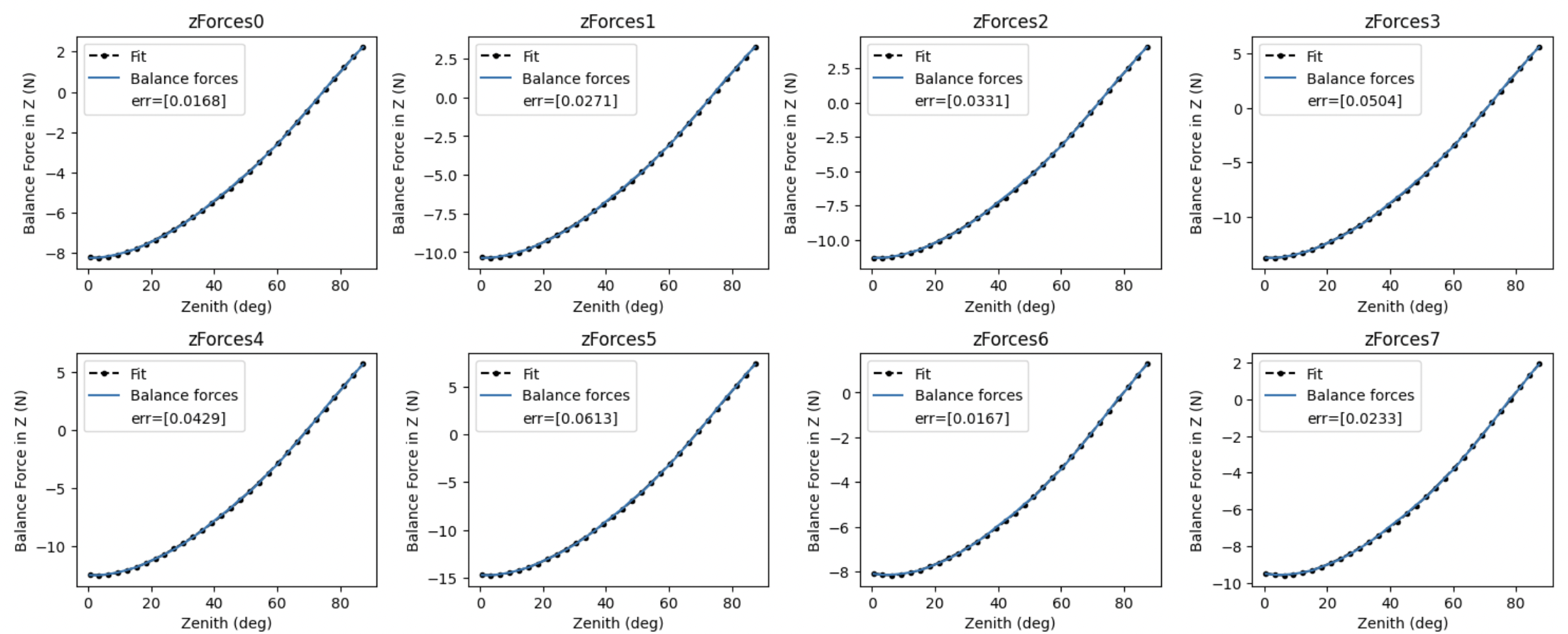
Balance forces: In this approach, we fit the balance forces offsets from the hardpoint correction system with a 5th-order polynomial. We add these coefficients to the existing LUT and generate a new .csv file with the new LUT. The CSV is created in the folder where you have the script.
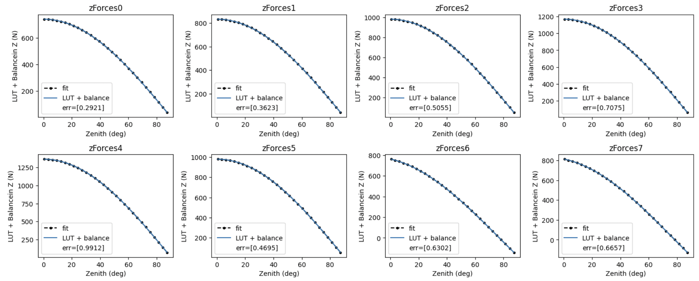
Applied forces: We look at the Applied forces minus the Static forces, which is equal to the LUT + Balance forces offsets. We make a fit on these and create a new LUT file, writing from scratch, without relying on the previous LUT.
After experimenting with both approaches, we found that the Applied forces approach is preferrable because it does not rely on previous LUT files. However, below we show how both approaches should give very similar results.
Another aspect to be considered is the hysteresis present in the system. Since we can’t correct for the hysteresis the updates that will be performed come from fitting the applied forces when doing a complete sweep of elevation angles, that is, from 0 degrees to 90 degrees and back to 0 degrees.
3 Fitting Balance Forces vs Fitting Applied Forces
We start by showing that we can use either approach to generate the updated LUT. When looking at the data retrieved on 2023-05-31 from 08:35 UTC to 09:05 UTC, with hardpoint corrections enabled (that is, the balance force system). Below is a plot of the two fits that are done to generate the updated LUT:
Balance forces

Applied Forces

The final LUT for the balance force approach is,

Which is approximately the same as the one obtained when using the applied forces approach (See below)

Now that we have shown that both approaches work, we will choose the “Balance force approach” as our baseline and will study the balance forces evolution ss we iteratively update the LUT.
4 LUT Iterative Improvement Results
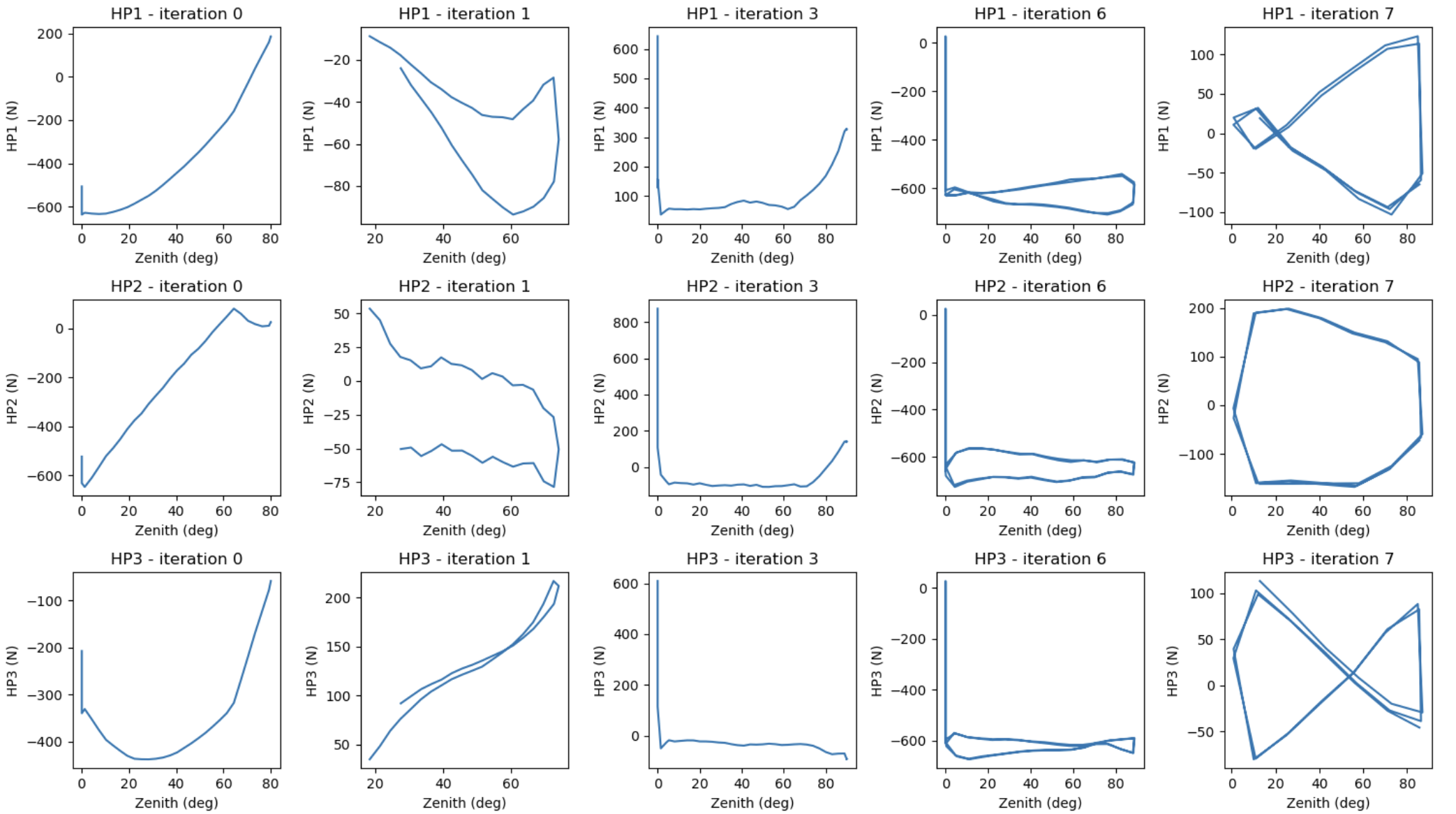
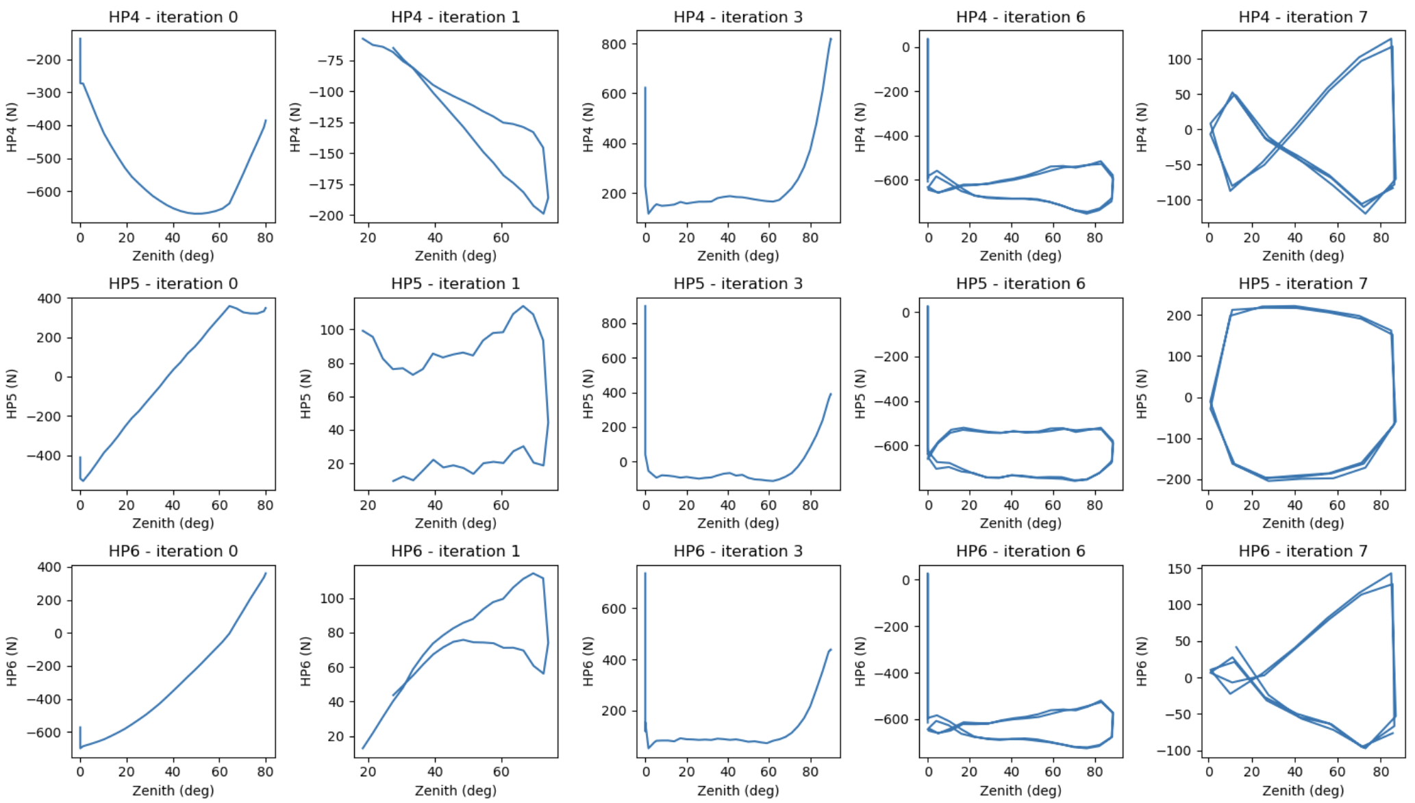
Now we want to look at the evolution of the Balance forces offsets after updating the LUT using the fits discussed in the previous section. In the plots below we see the change in the measured Hardpoint forces for five different iterations of the LUT. Note, that some of the iterations are missing because initially, we didn’t perform slews with the force balance system turned off, which allows us to quantify how much better is the LUT.


Before coming to any conclusions, it should be mentioned that the hysteresis of the system was not considered until iteration 6, hence up until then, the updates that were being performed failed to correct for the mean of the hysteresis loop and were instead being applied to only one of the slews.
We see that in the last two iterations, the hardpoint correction forces improved considerably. Let us recall that the “Rule of Thumb” for an open loop cell system is that we should expect about 1/1000 correction. Our mirror weighs 170,000 N. We should expect to get within 170N. It looks like we are within this range. If you actually RSS all the errors you get a much lower number, around 30 N per hardpoint. In light of these facts, the results of iteration 7 seem satisfactory.
5 Can we do any better?
The remaining last step on this iterative improvement approach that we hope to finalize soon, is to run a couple more improvement iterations and validate that we have effectively converged and that the hardpoint measured forces remain close to the current values.
6 Key considerations
When evaluating the LUT, it is important to perform slews with the force balance system turned on and turned off. When turned off, the hardpoint measured forces give us an idea of how much did we improve the LUT, while when turned on it allows us to gather data to improve the LUT again.
The polynomial fit should be done over a full slew (0 - 90 - 0 degrees) so that we account for the hysteresis of the system.
7 Instructions to update the LUT
7.1 Find EFD data to use for LUT improvement
Identify the Observation Block to be used for updating the LUT. Retrieve its start and end time.
Here is an example of how you can query and plot the data to find the elevations, in case you want to do it manually
start = Time('2023-05-31 08:35:0Z', scale='utc')
end = Time('2023-05-31 09:05:0Z', scale='utc')

# Retrieve elevations
elevations = await client.select_time_series(
   'lsst.sal.MTMount.elevation',
   ['actualPosition', 'timestamp'],
   start,
   end,
)
elevations = elevations['actualPosition'].resample('1T').mean()
elevations.plot()
plt.xlabel('Time (utc)')
plt.ylabel('elevation (deg)')
Once you have chosen the times you want to look at, write them down. You will need them for the next step.
7.2 LUT Improvement Script
Clone the ts_aos_utils repository that you can find here <https://github.com/lsst-ts/ts_aos_utils/>. Do the following
git clone https://github.com/lsst-ts/ts_aos_utils/
Go to the directory where you cloned the repository and run the script, which is located at
python/lsst/ts/aos/utils/scriptsRun the script m1m3_lut.py which will generate a LUT file in the same directory. You can run the script as follows
python3 M1M3LUT.py force_type start_time end_time axis --lut_path --polynomial_degree --resample_rate

# axis = ['X', 'Y', 'Z', 'XZ', 'XY', 'YZ', 'XYZ']
# force_type = ['Balance', 'Applied']
# --lut_path = path to the LUT file you want to improve, only needed if Balance approach is used
# --polynomial_degree = degree of the polynomial you want to fit the data to
# --resample_rate = resample rate of the data you want to use for the LUT improvement.
You will not have to change the polynomial degree or the resample rate. The default values are 5 and 1T respectively.
An example below:
python3 m1m3_lut.py 'Applied' '2023-05-31 08:35:0Z' '2023-05-31 09:05:0Z' 'XYZ'
Create a branch in the ts_config_mttcs repository and push your changes. You will have to ask the appropriate personnel for approval.
7.3 Updating the LUT in cRIO
Once the changes are approved into ts_config_mttcs, these changes need to be pulled into cRIO.
Ask for support from the appropriate personnel (Tiago / Petr) that will help update the LUT file, pulling it into cRIO and then cycling the M1M3 CSC to standby and bringing it back online. The new table will then be loaded during the start step.
8 Test rundown:
LUT Evaluation
Hardpoint corrections should be
OFFDo a 0 to 90 to 0 deg sweep.
LUT Improvement
Hardpoint corrections should be
ONFind times of the Observation Block in EFD data to use for LUT improvement
Run the script to generate a new LUT file for Z, Y and X axis. You can choose ‘Applied’ approach to start with.
Update the cRIO
Cycle M1M3 CSC to standby and bring it back to online. The new table is now loaded during start step.